Tutorial 2: nD Navigation and Hypersphere Slicing
Learn how to work with multi-dimensional data and understand Luxar’s unique nD visualization paradigm.
Goal
Create a 5D dataset (X, Y, Z, Time, Channel) and understand how hypersphere slicing enables intuitive nD navigation.
Core Concept: The Hypersphere Slicing Paradigm
The Challenge: You can’t display 5 dimensions on a 2D screen.
Traditional Solution (Dimension Reduction):
Use PCA, t-SNE, or UMAP to project 5D → 3D
Problem: Lose spatial relationships, can’t recover original dimensions
Luxar Solution (nD Slicing):
Display 3 dimensions (e.g., X, Y, Z)
Slice through 2 dimensions (e.g., Time, Channel)
Points visible based on distance in non-displayed dimensions
The Mathematics:
A point with radius R at position [x, y, z, t, c] is visible when:
If distance ≤ R, the effective radius in 3D is:
Visual Intuition:
Imagine a 3D sphere at (x, y, z, time=5, channel=2) with radius=3:
At time=5, channel=2: Full 3D sphere visible
At time=5.5, channel=2: Smaller circle visible (hypersphere cross-section)
At time=8, channel=2: Invisible (too far, outside hypersphere)
Side view (time dimension):

   time=2    time=5    time=8
     │         │         │
     │    ◄────R=3────►  │
     │   ╱             ╲ │
     ○  ◀──R_eff──▶     ○     ○ = slice positions
     │   ╲             ╱ │
     │    ╲───────────╱  │
     │         ●          │        ● = point center
             visible   invisible
Example: Time-Series Cell Tracking
from luxar.core import Dimensions, Dimension
from luxar.io import LuxarZarrCompiler
import numpy as np

# Define 4D space (3D + time)
dims = Dimensions([
    Dimension("X", unit="um", spatial=True, display=True),
    Dimension("Y", unit="um", spatial=True, display=True),
    Dimension("Z", unit="um", spatial=True, display=True),
    Dimension("Time", discrete=True, display=False, step=0.1),
])

# Create cell trajectories
n_cells = 100
n_timepoints = 50

with LuxarZarrCompiler('cells_4d.luxar.zarr') as compiler:
    scene = compiler.create_scene(dimensions=dims)

    for t in range(n_timepoints):
        # Cell positions at this timepoint
        positions_3d = cell_positions[t]  # Shape: (100, 3)

        # Add time coordinate
        time_values = np.full((n_cells, 1), t * 0.1)
        positions_4d = np.column_stack([positions_3d, time_values])  # Shape: (100, 4)

        # Add to scene
        scene.add_points(
            f"cells_t{t:03d}",
            positions_4d,
            colors=track_colors,  # Color by cell ID
            radii=5.0
        )
Why discrete=True for Time?
Tells Luxar to group by time in compound ordering
Makes time-series animation efficient (contiguous chunks)
Enables exact time selection (not interpolation)
Viewing 4D Data
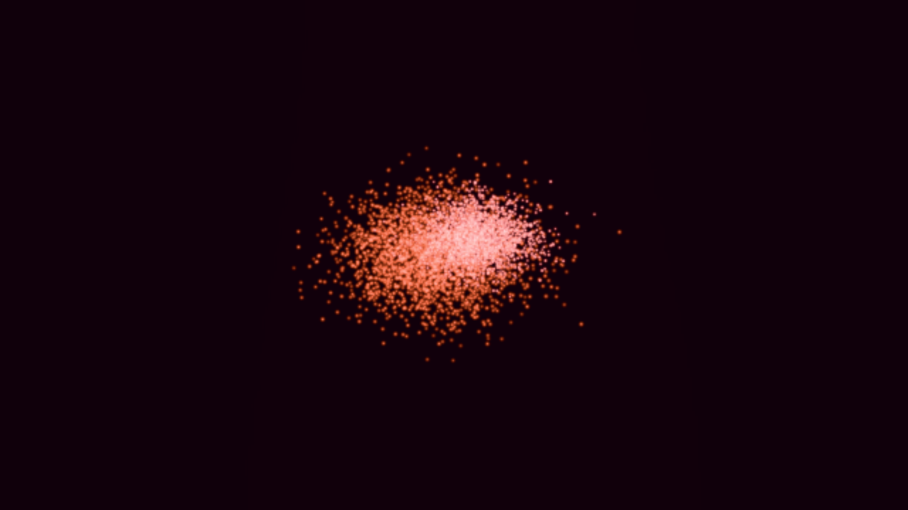
In the viewer:
Initial view: See all cells at time=0
Press 1: Select Time, the first non-displayed dimension (digit keys count only non-displayed dimensions)
Press ]: Navigate to time=1 (next timestep)
Observe: Cells appear/disappear based on hypersphere slicing
What you see:
Cells at exactly time=1: Full radius (bright, large)
Cells at time=0.9 or time=1.1: Smaller radius (dimmer, smaller)
Cells at time=5: Invisible (outside radius=5 in time dimension)
Advanced: Extend-to-All
Problem: Some data should be visible at all times/channels.
Example: Reference markers, coordinate axes, ROI boundaries
# Add reference grid visible at all times
grid_positions_3d = create_grid()  # Shape: (1000, 3)

# Extend to 4D by adding dummy time
grid_positions_4d = np.column_stack([
    grid_positions_3d,
    np.zeros((1000, 1))  # time=0 (will be extended)
])

scene.add_points(
    "reference_grid",
    grid_positions_4d,
    colors=(0.5, 0.5, 0.5),  # Gray
    radii=1.0,
    extend_to_all=["Time"]  # Visible at ALL times!
)
Result: Grid appears at every timepoint, providing spatial reference.
Categorical Dimensions
Use Case: Multi-channel fluorescence microscopy
dims = Dimensions([
    Dimension("X", unit="um", spatial=True, display=True),
    Dimension("Y", unit="um", spatial=True, display=True),
    Dimension("Z", unit="um", spatial=True, display=True),
    Dimension(
        "Channel",
        discrete=True,
        display=False,  # Non-displayed: at most 3 dims can be displayed
        categories=["DAPI", "GFP", "mCherry", "Cy5"]  # Named channels!
    ),
])
Benefits:
Navigate by channel name, not index
Viewer shows “DAPI” instead of “Channel 0”
Clearer data interpretation
Summary
Key Ideas:
nD data doesn’t need dimension reduction
Hypersphere slicing is intuitive and preserves all information
Discrete dimensions enable efficient grouping
Extend-to-all provides reference visibility
Categorical dimensions improve clarity
Next: Programmatic Server Creation - Create and test servers programmatically, or skip to Gaussian Splatting for Images for Gaussian splat fitting.