Tutorial 1: Creating Your First Scene

This tutorial walks through creating a complete Luxar scene from scratch, explaining each design decision and concept.

Goal

Create a 3D point cloud visualization with proper spatial ordering, compression, and interactive viewing.

What You’ll Learn:

Scene graph hierarchy and why it matters
Dimension definitions and their purpose
Spatial ordering benefits (compression and performance)
Encoding modes and when to use each
Viewing your data in the browser

Step 1: Import and Setup

import numpy as np
from luxar.core import Dimensions, Dimension
from luxar.io import LuxarZarrCompiler
from luxar.encoding import EncodingMode

Why these imports?

Dimensions: Define coordinate system (what each axis represents)
LuxarZarrCompiler: Progressive writer (no memory caching)
EncodingMode: Control compression vs precision tradeoff

Step 2: Create Sample Data

# Generate 100,000 random points in 3D
n_points = 100_000
positions = np.random.randn(n_points, 3).astype(np.float32) * 50  # 50 unit spread

# Colorful points (rainbow)
hue = np.linspace(0, 1, n_points)
colors = np.zeros((n_points, 3), dtype=np.float32)
colors[:, 0] = np.abs(np.sin(hue * np.pi * 2))      # Red
colors[:, 1] = np.abs(np.sin((hue + 0.33) * np.pi * 2))  # Green
colors[:, 2] = np.abs(np.sin((hue + 0.67) * np.pi * 2))  # Blue

Design Decision: Why float32?

GPU shaders use float32 internally
Smaller than float64, same visual precision
NumPy default is float64 - explicit conversion prevents waste

Step 3: Define Dimensions

dims = Dimensions([
    Dimension(
        name="X",
        unit="um",           # Micrometers (microscopy convention)
        spatial=True,        # This is a spatial dimension
        display=True,        # Show in 3D view
        range=[-100, 100]    # Hint for viewer bounds
    ),
    Dimension("Y", unit="um", spatial=True, display=True, range=[-100, 100]),
    Dimension("Z", unit="um", spatial=True, display=True, range=[-100, 100]),
])

Why define dimensions explicitly?

Viewer needs context: What do axes represent? What are the units?
Spatial ordering: Luxar knows which dimensions to use for Morton ordering
Navigation hints: Range and step guide viewer controls
Extensibility: Easy to add time, channel, etc. later

Spatial Flag Purpose:

spatial=True: Use in Morton/Hilbert ordering (physical space)
spatial=False: Discrete values (time, channel) - group don’t order

Step 4: Create Scene and Write Data

with LuxarZarrCompiler(
    'tutorial_scene.luxar.zarr',
    encoding_mode=EncodingMode.AUTO,  # Let Luxar choose encoding
    ordering_method="hilbert",        # Hilbert space-filling curve (best locality)
    enable_spatial_index=True,        # Calculate chunk bounds (CRITICAL for performance)
) as compiler:

    # Create scene with dimensions
    scene = compiler.create_scene(dimensions=dims)

    # Add points
    scene.add_points(
        name="rainbow_cloud",
        positions=positions,
        colors=colors,
        radii=2.0,  # Scalar! Broadcasted to all points automatically
    )

Encoding Mode Explanation:

AUTO: Analyzes data, chooses best encoding per array
- Positions: uint16 (50% size) - coordinates don’t need full float32 precision
- Colors: uint8 (75% size) - 256 levels per channel is plenty
- Radii: broadcast (99.9% size) - all points have same radius
PRECISION: float32 for everything (lossless, larger files)
MEMORY: Aggressive quantization (lossy, smallest files)

Spatial Ordering Benefit:

Without ordering:

Random access patterns
Poor compression (2-3×)
Slow queries (linear scan)

With Morton ordering:

Adjacent in space → adjacent in file
Excellent compression (6-10×)
Fast queries (chunk-based, ~200,000× faster)

Step 5: Verify and View

# Check what was created
import zarr
store = zarr.open('tutorial_scene.luxar.zarr', mode='r')
print(f"Scene dimensions: {store.attrs['scene_dimensions']}")
print(f"Nodes: {list(store.group_keys())}")

# Get compression stats
rainbow = store['rainbow_cloud']
# Note: Actual compression ratio depends on zarr store backend
print(f"Number of chunks: {rainbow['positions'].nchunks}")
print(f"Chunk shape: {rainbow['positions'].chunks}")

Then serve with the viewer:

luxar serve tutorial_scene.luxar.zarr --viewer

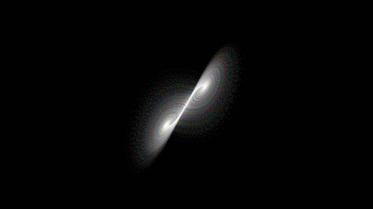
What happens when you open the viewer?

JavaScript loads scene metadata (dimensions, bounds)
Calculates initial visible chunks based on camera position
Fetches chunks from HTTP server (parallelized)
Caches in OPFS (persists across page reloads)
Decodes arrays (dequantize uint16 → float32)
Creates WebGL buffers
Renders at 60 FPS

Navigate the scene:

Mouse: Rotate, pan, zoom (orbit controls)
Keyboard: Arrow keys fly through space

Key Concepts Demonstrated

Scene Graph Hierarchy

The scene is a tree:

Scene (root)
└── rainbow_cloud (Points node)
    ├── positions/ (zarr array)
    ├── colors/ (zarr array)
    └── radii/ (broadcast scalar)

Why hierarchy?

Organize complex scenes (multiple datasets)
Apply transforms to groups
Control visibility per node

Progressive Writing

Critical Concept: Data is written immediately, not cached in memory.

dims = Dimensions.default_3d()
with LuxarZarrCompiler('scene.luxar.zarr') as compiler:
    scene = compiler.create_scene(dimensions=dims)

    # This writes to disk NOW, not at context exit
    scene.add_points("batch1", positions[:1000], colors[:1000])

    # Can process huge datasets in batches
    for i in range(0, n_points, batch_size):
        positions_batch = load_next_batch(i)  # Load only batch, not all
        scene.add_points(f"batch_{i}", positions_batch, ...)

    # Total memory usage: one batch size, not entire dataset!

Why this matters:

Handle TB datasets on GB machines
Never run out of memory
Write directly to compressed zarr chunks

Semantic Type Benefits

Luxar automatically optimizes encoding based on data semantics:

# Positions (COORDINATE semantic type)
# → Quantized to uint16 with min/max bounds
# → 50% size reduction, <0.1% precision loss

# Colors (COLOR semantic type)
# → uint8 for SDR (0-1 range)
# → geolog_perchannel_u16 for HDR (>1.0 values; decoded to float32)

# Radii (POSITIVE_SCALAR)
# → Uniform value broadcasted (99.9% savings)
# → or log quantization for varying radii

You don’t have to think about this - EncodingMode.AUTO handles it!

Next Steps

Tutorial 2: nD Navigation and Hypersphere Slicing - Add time and channel dimensions for nD navigation
Programmatic Server Creation - Create and test servers programmatically
Gaussian Splatting for Images - Fit Gaussian splats for compression and denoising
Tutorial 4: Performance Optimization - Optimize for billion-point datasets

Troubleshooting

Points not visible in viewer?

Check dimension ranges - are points outside bounds?
Check radii - too small to see? Try radii=10.0
Check colors - all black? Check color range [0, 1]

Slow to load?

Enable spatial ordering: enable_spatial_index=True (huge speedup)
Reduce chunk size: Smaller chunks = more granular loading
Check network: Localhost should be fast (~1ms), remote varies

File size too large?

Use EncodingMode.MEMORY instead of AUTO
Reduce point count (downsample if appropriate)
Check for duplicate data (use array references)