Tracking multi-colored cells using segmentation ensemble
This example shows using Ultrack to segment and track cells from a multi-color dataset. The data was provided by Richa Agrawal from The Lammerding Lab.
The individual channels can have a significant dynamic range between the fluorescence intensities. This becomes an issue when applying an off-the-shelf deep learning segmentation model, in this case, Cellpose.
Therefore, we use an ensemble of segmentation models, employing:
Cellpose: which obtains very accurate segmentation but misses a few dim cells;
Watershed: This is less accurate, but we have greater control and can easily tune to detect most cells.
We combine the segmentation from different channels and methods in the segment contour space and let Ultrack pick the most accurate while tracking the cells. We will describe this in more detail down below.
We use out-of-memory storage of the image data to minimize the required resources. Therefore, this jupyter notebook can be executed in Google Colab.
When running this example on Google Colab, you can get the best performance using a GPU.
To do that, change runtime to GPU by clicking on Runtime -> Change runtime type -> Hardware Accelerator -> GPU.
And you must uncomment the lines below to install the additional packages and restart the notebook.
[1]:
# Required if running on Google Colab
# !pip install pyift gurobipy cucim cellpose "napari[all]"
# !pip install ultrack
When using Colab, change the variable to COLAB = True to avoid using napari and to connect it to your drive.
[2]:
# Change this variable if using Colab to load your data
COLAB = False
if COLAB:
from google.colab import drive
drive.mount('/content/gdrive')
# Setting up gurobi
import os
import gurobipy as gp
os.environ["GRB_LICENSE_FILE"] = "/content/gdrive/YOUR/DIRECTORY/gurobi.lic" # make sure to change to your gurobi.lic WSL file
gp.Model() # testing if it works
[3]:
# importing required packages
import pickle
from pathlib import Path
from typing import Optional
from pathlib import Path
import napari
import dask.array as da
import numpy as np
import pandas as pd
import scipy.ndimage as ndi
import seaborn as sns
import zarr
from tifffile import imread, imwrite
from tqdm import tqdm
from IPython.display import display
from napari.utils.notebook_display import nbscreenshot
from numpy.typing import ArrayLike
from ultrack import track, to_tracks_layer, tracks_to_zarr # to_trackmate,
from ultrack.utils import labels_to_contours
from ultrack.config import MainConfig
from ultrack.imgproc import normalize
from ultrack.imgproc.segmentation import reconstruction_by_dilation, Cellpose
from ultrack.utils.array import array_apply, create_zarr
from ultrack.utils.cuda import import_module, to_cpu, torch_default_device
from rich import print
from pyift.shortestpath import watershed_from_minima
from skimage.segmentation import relabel_sequential
from skimage.filters import threshold_otsu
import skimage.morphology as morph
try:
import cupy as xp
except ImportError:
import numpy as xp
We implement some additional functions to remove the background signal, apply the watershed using an otsu threshold of the input image plus the detected regions from Cellpose and demonstration function to plot the cells movement.
[4]:
# helper functions
def remove_background(image: ArrayLike, sigma=15.0) -> ArrayLike:
"""
Removes background using morphological reconstruction by dilation.
Reconstruction seeds are an extremely blurred version of the input.
Parameters
----------
imgs : ArrayLike
Raw image.
Returns
-------
ArrayLike
Foreground image.
"""
image = xp.asarray(image)
ndi = import_module("scipy", "ndimage")
seeds = ndi.gaussian_filter(image, sigma=sigma)
background = reconstruction_by_dilation(seeds, image, iterations=100)
foreground = np.maximum(image, background) - background
return to_cpu(foreground)
def watershed_segm(
frame: ArrayLike,
aux_labels: ArrayLike,
min_area: int,
) -> tuple[ArrayLike, ArrayLike]:
"""
Detects foreground using Otsu threshold and auxiliary labels,
and execute watershed from minima inside that region.
Parameters
----------
frame : ArrayLike
Images as an Y,X array.
aux_labels : ArrayLike
Auxiliary labels are used to detect the foreground.
min_area : int
Minimum size to be considered a cell.
Returns
-------
ArrayLike
Watershed segmentation labels.
"""
disk3 = ndi.generate_binary_structure(frame.ndim, 3)
frame = frame.astype(np.float32)
frame = ndi.gaussian_filter(frame, 3.0)
det = frame > (threshold_otsu(frame) * 0.75) # making otsu less conservative
det = np.logical_or(det, np.asarray(aux_labels) > 0)
det = morph.remove_small_objects(det, min_area)
det = ndi.binary_closing(det, structure=disk3)
edt = ndi.distance_transform_edt(det)
labels = relabel_sequential(watershed_from_minima(-edt, det, H_minima=2.0)[1])[0]
return labels
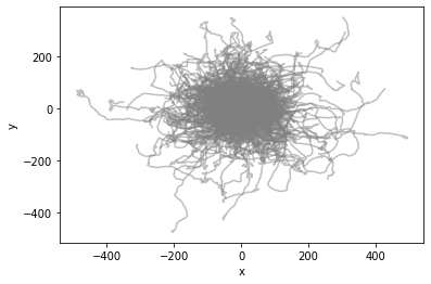
def plot_tracks(tracks_df: pd.DataFrame) -> None:
"""Center tracks at their initial position and plot them.
Parameters
----------
tracks_df : pd.DataFrame
Tracks datafarame sorted by `track_id` and `t`.
Returns
-------
pd.DataFrame
Centered dataframe.
"""
centered_df = tracks_df.copy()
centered_df[["y", "x"]] = centered_df.groupby(
"track_id",
as_index=False,
)[["y", "x"]].transform(lambda x: x - x.iloc[0])
# sanity check
assert (centered_df[centered_df["t"] == 0][["y", "x"]] == 0).all().all()
pallete = sns.color_palette(["gray"], len(centered_df["track_id"].unique()))
sns.lineplot(
data=centered_df,
x="x",
y="y",
hue="track_id",
palette=pallete,
legend=False,
alpha=0.5,
sort=False,
estimator=None,
)
return centered_df
Finally, we download the data and load it. As with the other examples, time is the leading dimension. To decrease the memory usage we store our intermediate data in zarr arrays, which behave just like a numpy array, but the data is compressed and saved in the disk.
[5]:
!wget http://public.czbiohub.org/royerlab/ultrack/multi-color-cytoplasm.tif
--2024-05-31 08:53:34-- http://public.czbiohub.org/royerlab/ultrack/multi-color-cytoplast.tif
Resolving public.czbiohub.org (public.czbiohub.org)... 10.79.124.99
Connecting to public.czbiohub.org (public.czbiohub.org)|10.79.124.99|:80... connected.
HTTP request sent, awaiting response... 200 OK
Length: 2488361461 (2.3G) [image/tiff]
Saving to: ‘multi-color-cytoplast.tif.1’
multi-color-cytopla 100%[===================>] 2.32G 72.3MB/s in 33s
2024-05-31 08:54:07 (72.2 MB/s) - ‘multi-color-cytoplast.tif.1’ saved [2488361461/2488361461]
[6]:
# image path, change this
# (T, Y, X, C) data, where T=time, Y, X =s patial coordinates and C=channels
img_path = Path("multi-color-cytoplasm.tif")
# optional, useful for a quick look
# for all frames `n_frames = None`
n_frames = None
imgs = imread(img_path)
chunks = (1, *imgs.shape[1:-1], 1) # chunk size used to compress data
if n_frames is not None:
imgs = imgs[:n_frames]
if not COLAB:
viewer = napari.Viewer()
viewer.window.resize(1800, 1000)
layers = viewer.add_image(imgs, channel_axis=3, name="raw")
display(nbscreenshot(viewer))
for l in layers:
l.visible = False
print(f"Image size (T, Y, X, C) = {imgs.shape}")

Image size (T, Y, X, C) = (300, 1440, 1920, 3)
As seen above, the image contains a lot of background noise. So we use our remove_background helper function to remove it. Additionaly, we manually normalize the image to the range of 0 to 1 as required by Cellpose and take the square root of it (gamma=0.5), we do this to decrease the dynamic range, boosting a bit Cellpose’s performance.
[7]:
foreground = create_zarr(imgs.shape, imgs.dtype, "foreground.zarr", chunks=chunks, overwrite=True)
array_apply(
imgs,
out_array=foreground,
func=remove_background,
sigma=15.0,
axis=(0, 3),
)
normalized = create_zarr(imgs.shape, np.float16, "normalized.zarr", chunks=chunks, overwrite=True)
array_apply(
foreground,
out_array=normalized,
func=normalize,
gamma=0.5,
axis=(0, 3),
)
normalized = da.from_zarr(normalized, chunks=chunks)
if not COLAB:
viewer.add_image(imgs, channel_axis=3, name="raw", visible=False)
viewer.add_image(foreground, channel_axis=3, name="foreground", visible=False)
viewer.add_image(normalized, channel_axis=3, name="normalized")
display(nbscreenshot(viewer))
Applying remove_background ...: 100%|██████████| 900/900 [00:33<00:00, 26.91it/s]
Applying normalize ...: 100%|██████████| 900/900 [01:06<00:00, 13.54it/s]

The cells look much clearer now. Next, we apply Cellpose to each channel individually because we don’t have a model for 3-channel cytoplasm-labeled data. Defining a heuristic to fuse the segments from different channels can be challenging, so we use the labels_to_edges function to convert and combine each segment into contours. During tracking Ultrack compares the segmentation using the contour map and selects non-overlapping segments to the tracking solution.
[8]:
cellpose_labels = create_zarr(imgs.shape, np.uint16, "cellpose_labels.zarr", chunks=chunks, overwrite=True)
array_apply(
normalized,
out_array=cellpose_labels,
func=Cellpose(model_type="cyto2", device=torch_default_device()),
axis=(0, 3),
tile=False,
normalize=False,
)
# using dask (da = dask.array) to make a lazy array
cellpose_labels = da.from_zarr(cellpose_labels, chunks=chunks)
merged_labels = cellpose_labels.max(axis=-1)
if not COLAB:
layer = viewer.add_labels(merged_labels, name="cellpose_labels")
display(nbscreenshot(viewer))
layer.visible = False # shutting if off
Applying Cellpose ...: 100%|██████████| 900/900 [12:47<00:00, 1.17it/s]

Some of the dimmer cells are not detected by Cellpose, so we apply a custom routine using watershed to provide an auxiliar set of segments. We combine the watershed and Cellpose segmentations as we did with the segmentation from different channels.
[9]:
# ws_labels = watershed_segm(normalized, cellpose_labels, min_area=250)
ws_labels = create_zarr(imgs.shape, np.int32, "ws_labels.zarr", chunks=chunks, overwrite=True)
array_apply(
normalized,
cellpose_labels,
out_array=ws_labels,
func=watershed_segm,
min_area=250,
axis=(0, 3),
)
ws_labels = da.from_zarr(ws_labels, chunks=chunks)
# Combining watershed results
detection, contours = labels_to_contours(
[cellpose_labels[..., c] for c in range(cellpose_labels.shape[-1])] +\
[ws_labels[..., c] for c in range(ws_labels.shape[-1])],
sigma=5.0,
detection_store_or_path=zarr.TempStore(),
edges_store_or_path=zarr.TempStore(),
)
Applying watershed_segm ...: 100%|██████████| 900/900 [06:19<00:00, 2.37it/s]
<ipython-input-9-e45de74e19eb>:14: DeprecationWarning: Argument detection_store_or_path is deprecated, please use foreground_store_or_path instead.
detection, contours = labels_to_contours(
Converting labels to contours: 100%|██████████| 300/300 [00:14<00:00, 21.04it/s]
Finally, we can track the cells. Ultrack parameters are defined in the MainConfig class. Each step contains its own parameters in a subconfiguration (e.g., config.linking_config). These parameters were found by inspecting the tracking results.
The configuration documentation can be found here.
[10]:
config = MainConfig()
n_workers = 1 if COLAB else 8
# Candidate segmentation parameters
config.segmentation_config.n_workers = n_workers
config.segmentation_config.min_area = 200
config.segmentation_config.min_frontier = 0.01
# Setting the maximum number of candidate neighbors and maximum spatial distance between cells
config.linking_config.max_neighbors = 5
config.linking_config.max_distance = 40
config.linking_config.n_workers = n_workers
config.linking_config.z_score_threshold = 3.0
# Tracking integer linear programming (ILP) parameters
config.tracking_config.division_weight = -0.01
config.tracking_config.disappear_weight = -2
config.tracking_config.appear_weight = -0.1
config.tracking_config.solution_gap = 0.0
## OPTIONAL, uncomment to use these options
## ILP processing window size.
## It reduces memory usage while asserting continuity in the tracks.
# config.tracking_config.window_size = 15
# config.tracking_config.overlap_size = 3
# config.tracking_config.solution_gap = 0.01
print("ultrack config")
print(config)
ultrack config
MainConfig( data_config=DataConfig(working_dir=PosixPath('.'), database='sqlite', address=None, n_workers=1), segmentation_config=SegmentationConfig( threshold=0.5, min_area=200, max_area=1000000, min_frontier=0.01, anisotropy_penalization=0.0, max_noise=0.0, ws_hierarchy=<function watershed_hierarchy_by_area at 0x7f2eaaba8a60>, n_workers=8 ), linking_config=LinkingConfig( n_workers=8, max_neighbors=5, max_distance=40, distance_weight=0.0, z_score_threshold=3.0 ), tracking_config=TrackingConfig( appear_weight=-0.5, disappear_weight=-0.1, division_weight=-0.01, dismiss_weight_guess=None, include_weight_guess=None, window_size=15, overlap_size=3, solution_gap=0.0, time_limit=36000, method=0, n_threads=-1, link_function='power', power=4, bias=-0.0 ) )
We track the cells using the previously set config parameters, the combined cell detection and contour maps. Additionaly, we provide the processed raw data (normalized) so the tracking takes into account the segments intensity.
[11]:
track(
config,
detection=detection,
edges=contours,
images=[normalized[..., c] for c in range(normalized.shape[-1])],
overwrite=True
)
tracks_df, lineage_graph = to_tracks_layer(config)
tracking_labels = tracks_to_zarr(config, tracks_df)
if not COLAB:
viewer.add_labels(tracking_labels, name="ultrack labels")
viewer.add_tracks(tracks_df[["track_id", "t", "y", "x"]], graph=lineage_graph, name="ultracks")
display(nbscreenshot(viewer))
<ipython-input-11-ba8137ac3995>:1: DeprecationWarning: Argument detection is deprecated, please use foreground instead.
track(
Adding nodes to database: 100%|██████████| 300/300 [02:17<00:00, 2.19it/s]
Linking nodes.: 100%|██████████| 299/299 [00:16<00:00, 18.65it/s]
Using Gurobi solver
Solving ILP batch 0
Constructing ILP ...
Solving ILP ...
Saving solution ...
Done!
Using Gurobi solver
Solving ILP batch 2
Constructing ILP ...
Solving ILP ...
Saving solution ...
Done!
Using Gurobi solver
Solving ILP batch 4
Constructing ILP ...
Solving ILP ...
Saving solution ...
Done!
Using Gurobi solver
Solving ILP batch 6
Constructing ILP ...
Solving ILP ...
Saving solution ...
Done!
Using Gurobi solver
Solving ILP batch 8
Constructing ILP ...
Solving ILP ...
Saving solution ...
Done!
Using Gurobi solver
Solving ILP batch 10
Constructing ILP ...
Solving ILP ...
Saving solution ...
Done!
Using Gurobi solver
Solving ILP batch 12
Constructing ILP ...
Solving ILP ...
Saving solution ...
Done!
Using Gurobi solver
Solving ILP batch 14
Constructing ILP ...
Solving ILP ...
Saving solution ...
Done!
Using Gurobi solver
Solving ILP batch 16
Constructing ILP ...
Solving ILP ...
Saving solution ...
Done!
Using Gurobi solver
Solving ILP batch 18
Constructing ILP ...
Solving ILP ...
Saving solution ...
Done!
Using Gurobi solver
Solving ILP batch 1
Constructing ILP ...
Solving ILP ...
Saving solution ...
Done!
Using Gurobi solver
Solving ILP batch 3
Constructing ILP ...
Solving ILP ...
Saving solution ...
Done!
Using Gurobi solver
Solving ILP batch 5
Constructing ILP ...
Solving ILP ...
Saving solution ...
Done!
Using Gurobi solver
Solving ILP batch 7
Constructing ILP ...
Solving ILP ...
Saving solution ...
Done!
Using Gurobi solver
Solving ILP batch 9
Constructing ILP ...
Solving ILP ...
Saving solution ...
Done!
Using Gurobi solver
Solving ILP batch 11
Constructing ILP ...
Solving ILP ...
Saving solution ...
Done!
Using Gurobi solver
Solving ILP batch 13
Constructing ILP ...
Solving ILP ...
Saving solution ...
Done!
Using Gurobi solver
Solving ILP batch 15
Constructing ILP ...
Solving ILP ...
Saving solution ...
Done!
Using Gurobi solver
Solving ILP batch 17
Constructing ILP ...
Solving ILP ...
Saving solution ...
Done!
Using Gurobi solver
Solving ILP batch 19
Constructing ILP ...
Solving ILP ...
Saving solution ...
Done!
Exporting segmentation masks: 100%|██████████| 300/300 [00:06<00:00, 46.52it/s]

For demonstration purposes we plot the displacement of the cells using the starting position as the origin.
[12]:
centered_df = plot_tracks(tracks_df)
We also export the results into the disk.
[13]:
if COLAB:
data_dir = img_path.parent
img_name = img_path.name.removesuffix(".tif")
results_dir = data_dir / img_name
results_dir.mkdir(exist_ok=True)
else:
results_dir = Path(".")
tracks_df.to_csv(results_dir / "tracks.csv", index=False)
imwrite(results_dir / "segments.tif", tracking_labels)
imwrite(results_dir / "cellpose_segments.tif", merged_labels)
# to_trackmate(config, results_dir / "tracks.xml", overwrite=True)
print(f"Saved results into {results_dir}")
Saved results into .